What can we learn from big whorls and little buoys? (part 2)
How can we study these smaller whorls at the smaller and smaller scales that can influence the movement of patches of nutrients, light, or both? With small buoys!
Analysis of the smaller whorls
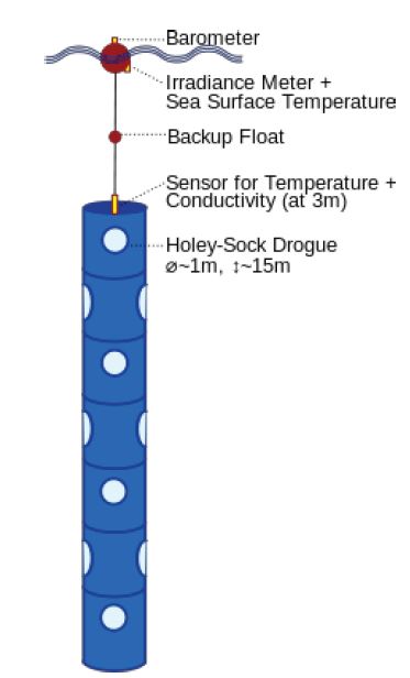
These buoys are part of international Iridium Surface Velocity Program, so we call them iSVPs. Purchased by Environment Canada`s Department of Fisheries and Oceans and manufactured by MetOcean in Halifax, Green Edge 2016 is deploying 6 of these iSVPs in Baffin Bay. One will be placed on an ice floe, rather than directly into the water. Each buoy consists of a small spherical surface unit about 75 cm in diameter and a holey sock drogue (because it`s like an old sock with holes!) that hangs down from 3 to 18 m deep into the ocean, catching the surface currents, much like a kite in the wind. The data from these buoys is sent by satellite phone to a data center near Halifax. The data will be used to see how well computer models of ocean circulation predict both the big whorl of the counter-clockwise circulation of Baffin Bay, as well as the smaller whorls…and subsequently make these predictions better.
Smaller Whorls Revealed
Three iSVP buoys have been deployed from the CCGS Amundsen during Leg 1 of the expedition.
- The first was deployed from the 500 deck, splashing down 7 m into the water (short of the 10 m maximum distance recommended by the manufacturer). It stopped operating soon after deployment, so subsequent deployments have been made gently from only 30 cm above the ocean surface from the Amundsen`s Zodiac.

- The second iSVP (Figure 1 below : GE_09: right, blue pin for starting location) was deployed on July 1st in open water about 700 m from the ship from a Zodiac. The 4.5 day trajectory was plotted in Google Earth from data transmitted once per hour. GE_09 started with a quick demonstration of smaller whorls created by surface tides. It took about 12.5 hours for GE_09 to make each loop, which corresponds to the period of a semi-diurnal (twice daily or M2) tide. From the geometry of these “tidal ellipses”, we can estimate the direction and strength of tidal currents. For example, each loop is about 3.5 km (longest axis) by 1.5 km (shorter axis), which represents a tidal current of about 17 cm per second or 0.34 knots. (figure 2 below) GE_09 then quickly drifted southward on July 4th, probably due to a period of much stronger wind-driven currents. As the winds subsided, the buoy again began tracing more of these tidal loops superimposed on a southward surface current, spreading out the tidal loops a bit. Including the five loops, it has travelled 83 km in 4.5 days, or almost 8 km per day. The net southward movement was 35 kilometers.


- The third iSVP buoy (Figure 1 above: GE_01 : left, white pin for starting location) was deployed a day later (July 2nd) directly on an ice floe. At this point, the buoy is simply plotting the motion of the ice floe. The small scale tidal ellipses are less evident due to the size of the ice floe (more than 1 km across), but they are still visible. Similar to iSVP GE_09, there was quick southward displacement on July 4th (figure 3 below). It travelled southward 46 km at about 13 km / day, thus farther and faster than the GE_09. This is because of the wind pushes the ice like a big sail. As the ice floe melts, we hope the holey sock drogue won`t get tangled in the ice and that GE_01 can continue to function as an ocean surface drifter.


The size of the eddies observed with both iSVPs (3-5 km diameter) is consistent with the theory of geophysical fluid dynamics (the “2nd baroclinic mode of the Rossby Radius of Deformation”), for our latitude (70° N) and the observed vertical profiles of temperature and salinity (weakly stratified, small buoyancy frequency N) which determine the pressure gradients. The Rossby radius describes the “natural scale” of features such as eddies, fronts, and boundary currents. So, theory agrees with observation of these smaller whorls. These small scale eddies are common in the Arctic given its latitude (the geostrophic part) and weak stratification (small N = buoyancy frequency part).
“And so on to viscosity“
While the transition from larger to smaller whorls involves the transfer of kinetic energy to smaller scales, the fate of the smallest whorls is to dissipate energy completely into heat through viscous forces, sort of like rubbing your hands together creates heat through friction. On this blog, see The Silent Scale which describes an instrument called the SCAMP that is being used to study this final step in the cascade of energy dissipation in the ocean, the tiniest whorls.