Gliders: Gliding close to and under the ice! (Part 2)
Since we deployed our two gliders, “Qala1” and “Qala2”, we are learning a lot “on the job”, i.e. we are building a strong experience by making minor beginner’s mistakes. We need to deal with a lot of files, and just a small tiny comma forgotten here or there is ending up in a mission’s abort! But the glider’s software is also very well written and is rather foolproof. Coupled with strong hotline from glider’s provider (Teledyne Webb Research) and our friends at LOCEAN, Ocean Tracking Network (OTN) and their glider group, we feel more and more confident with our flights.
The Marginal Ice Zone is very dynamic!
The MIZ (Marginal Ice Zone) is a very dynamic zone, and as such, we have to fly our gliders in relatively strong currents. I mean strong for a glider. Indeed, these vehicles are not moving very fast in the water, they are not designed for that (but the good side of it is their very long autonomy!).
A good rule of thumb for estimating is a horizontal velocity of 1 km/hour or roughly 20 to 25 km/day. So flying into a 10 cm/s current (i.e. 0.36 km/hour or nearly 9km/day) will impact a glider flight significantly. Also, when the glider is surfacing to get a GPS fix (to correct its dead-reckoned location), to upload new configuration files or to download a sub-sample of its measurements files, it drifts with surface winds. In the end, we take a look at our glider paths, we feel like we walk a young dog at the end of our leash!
Thanks to software from our friends at OTN, the glider paths can be visualized in Google Earth, along with satellite images of the ice, and are annotated to keep useful piloting information at our fingertips, including the estimated current direction and speed (the thin green line at each vertex on the figure below).
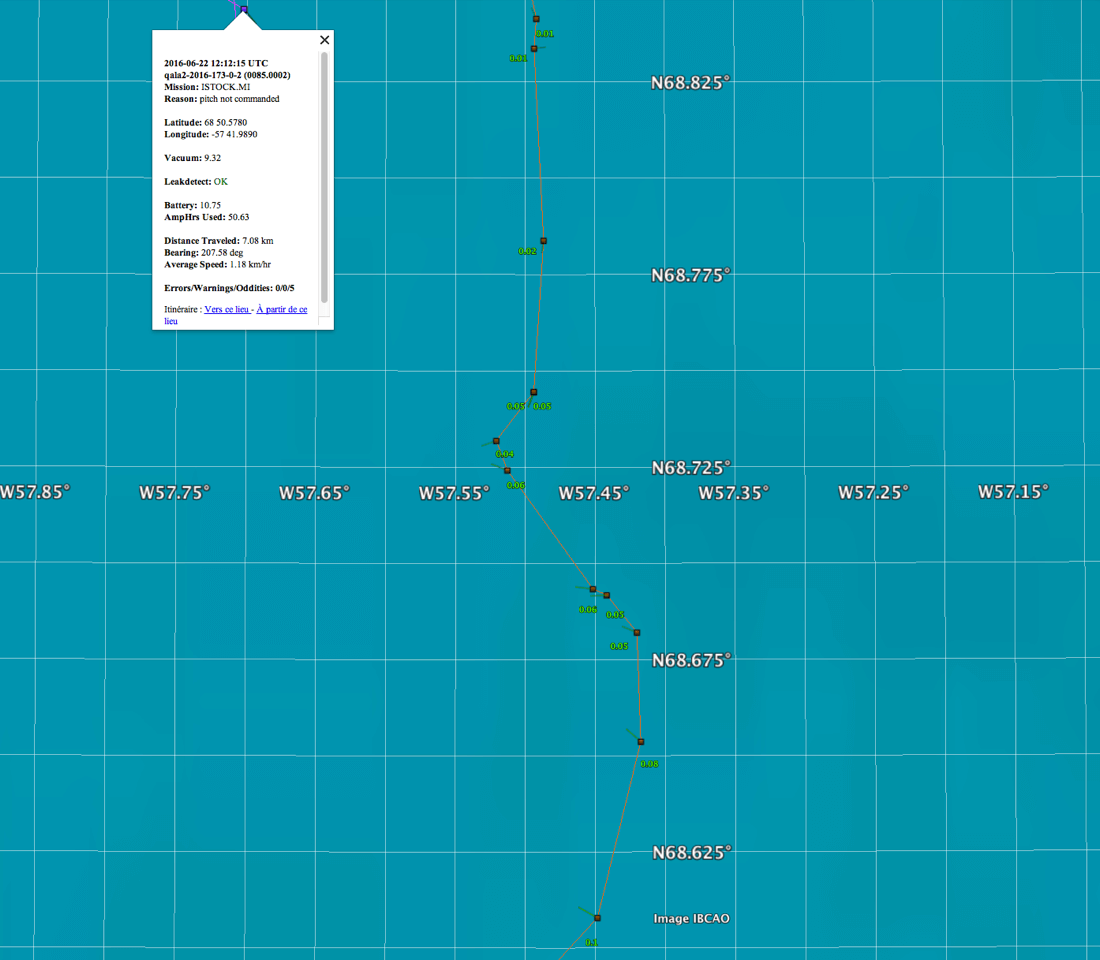
Picture of a typical glider track
All the deployment details, like maps, data sets, gliders health parameters etc. can also be found on the EGO web site, onto which both Qala1 and Qala2 are reporting. See an example on the figures below (on each site, you can navigate from plot to plot by clicking on “next plot” or “previous plot”).

Example of figures that can be found on the EGO web site.
Then came the time to try our first under ice mission!
Again, approaching the MIZ and its west part is itself very challenging, as the MIZ can move 10 km westward per day! (the most drastic event was a 100 km westward move in one day). Our gliders are travelling 20 km per day, you can see why we call this challenge “chasing the MIZ”! But after few days of trials, we were there, close to the MIZ, and we sent our glider under the ice. The first hours of silence were rather stressful, we kept on wondering if we made this little easily done mistake that would compromise the glider’s safety!
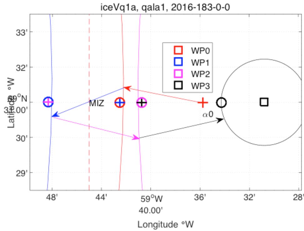
Eric spent a lot of time writing a computer code (in MatLab, from MathWorks©) to quickly design a mission, i.e. by setting several waypoints that would be used as targets by the glider. Usually, a glider is aiming at a waypoint, and considers it is achieved when close enough to it, say for example in a radius of 100 m or 200 m from it. But here, we cannot surface under the ice to get a GPS fix and correct any propagated error in the dead-reckoned location (i.e. where the glider thinks it is). In this way Eric’s code is setting waypoints with very large radii, in the order of few tens of km, to work with arrival lines rather than with arrival points. And this makes a big difference, as the heading errors under the ice, i.e. the errors that can’t be corrected because of the lack of GPS fix are finally not that important.
For example, our first glider that traveled under the ice came back approximately 6 km North of where we were expecting it – approximately 30 degrees of heading error! –
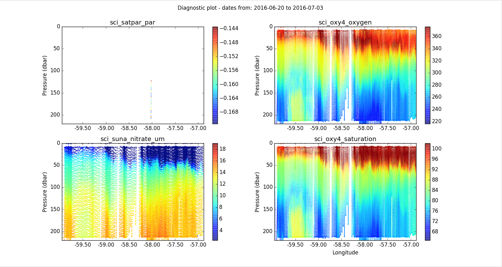
Observations from our science sensors
On the preliminary results reported below, we can see the longitudinal evolution of the phytoplankton bloom, less intense and less deep under the ice or in the MIZ, and more intense and deeper in the open water part of the glider’s tracks. The water masses are also different between these two sites of interest. Indeed, the water is colder and fresher under the ice, warmer and saltier in the open water zone. The nutrients are also more depleted where the bloom is more intense, which makes sense as the phytoplankton use these nutrients to grow. Also, they produce oxygen during their photosynthesis, and indeed, we can see the dissolved oxygen is more intense where the bloom is more advanced. A more thorough data analysis will provide us with time and regional variation of this trend.
Note the lack of light levels data (“sci_satpar_par” on the top / left hand side part of the 3rd figure, as the light sensor has been turned off – See part #1 of this post).
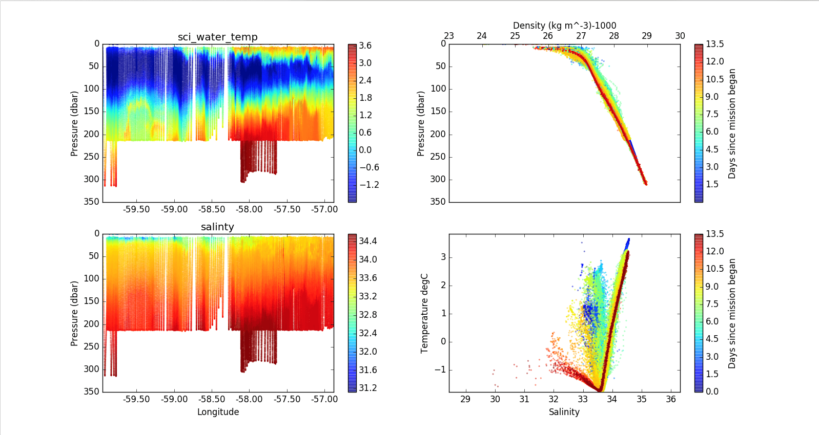
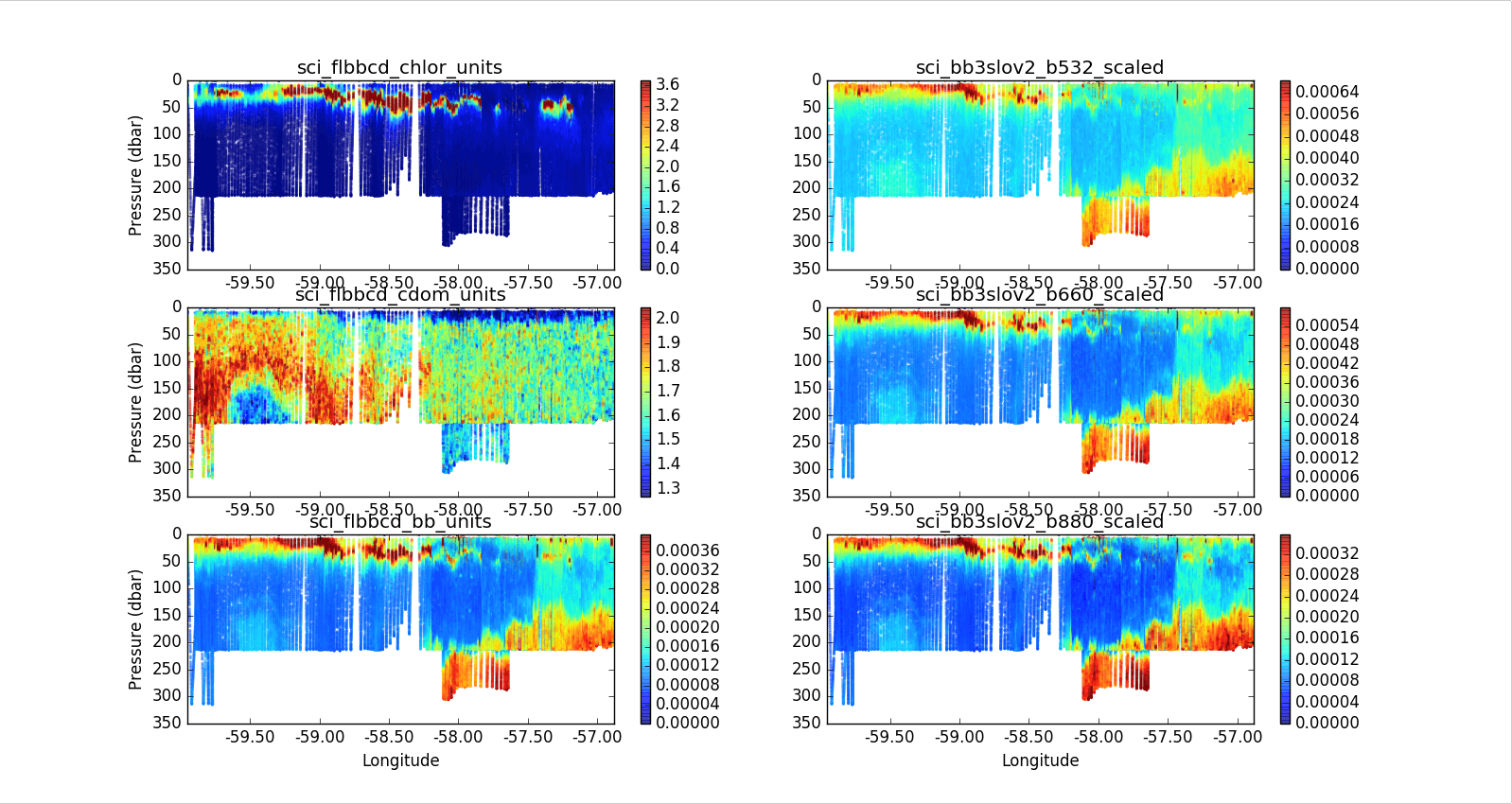
Below is a very preliminary set of plots from the first under-ice mission of Qala1. Note that the ranges of the color scales are different, for example, the Chlorophyll-a concentration is more than three times less than in open waters (1.05 a.u. instead of 3.6 a.u.).
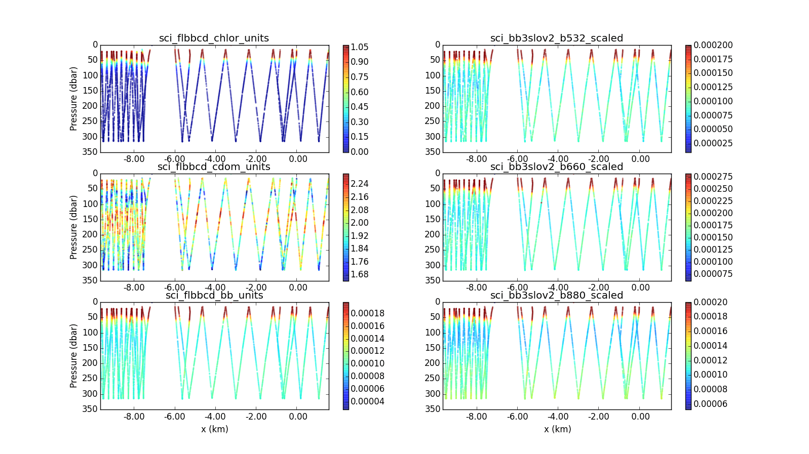
The under ice part of the mission is the positive side of the x axis (on the right side of the “zero”). The negative side of the x axis (on the left side of the “zero”) corresponds to the part of the mission that took place in the MIZ.
Qala1 was recovered on 9 July, and Qala2 on 10 July, both close to the MIZ. Just before its recovery, Qala2 was even flying in an area characterized with a fresher water layer due to more advanced melting ice. This layer of water is less dense. Say it in another way: the glider is more dense, or more heavy, so it was pretty hard to find, as it was sitting much lower at the sea surface, see the picture below! The gliders come with a strobe light, that we can switch on to help finding them during recovery operations, but here, even at 2am, the sun shines, so it was not very helpful (we still did it!). At the end, getting GPS fixes much more often made it possible to locate the glider among large ice chunks. We are very happy to have flown our gliders where no other gliders have been before!
