Green Edge, Green Leads!

« Green Edge is also partly motivated by the recent discovery that phytoplankton blooms may occur more extensively and more often under the ice-pack. » (http://www.greenedgeproject.info/rationale.php)

In the frame of the GreenEdge project, divers instruments have been deployed to evaluate the constituents of the water column and observe, among others, phytoplankton blooms. One approach consists to evaluate the colour of the water surface, namely, the fraction of the total incoming light reflected by the water surface as a function of wavelength, referred to as ‘ocean colour’. The principal concept of ocean colour relies on the fact that the nature and concentration of the water constituents affect the absorption and scattering of the incoming light and, subsequently, the colour of the water. Variations in ocean colour thus reflect variations in organic, inorganic, particulate and dissolved materials present in the water. For instance, satellite remote sensing ocean colour images can depict variations in total chlorophyll a (Chla) pigment concentration, a proxy for phytoplankton biomass. Chla preferentially absorbs red and blue light and scatters in the green spectral region. Hence by looking at the ocean colour as a function of wavelength, one may estimate the water constituents and their concentration. In addition, the spectral shape of the water reflectance may also be used to classify the water masses in different optical water classes. For instance, in a recent paper Melin and Vantrepotte (2015) derived a set of 16 optical water classes over global coastal waters based on the spectral shape of satellite retrieved water reflectance spectra. The 16 optical classes covered conditions from very turbid waters with divers concentrations of Chla to clear blue oligotrophic waters. In the Baffin Bay, the authors found a larger occurrence of low to moderately turbid waters with a peak in the blue spectral region.

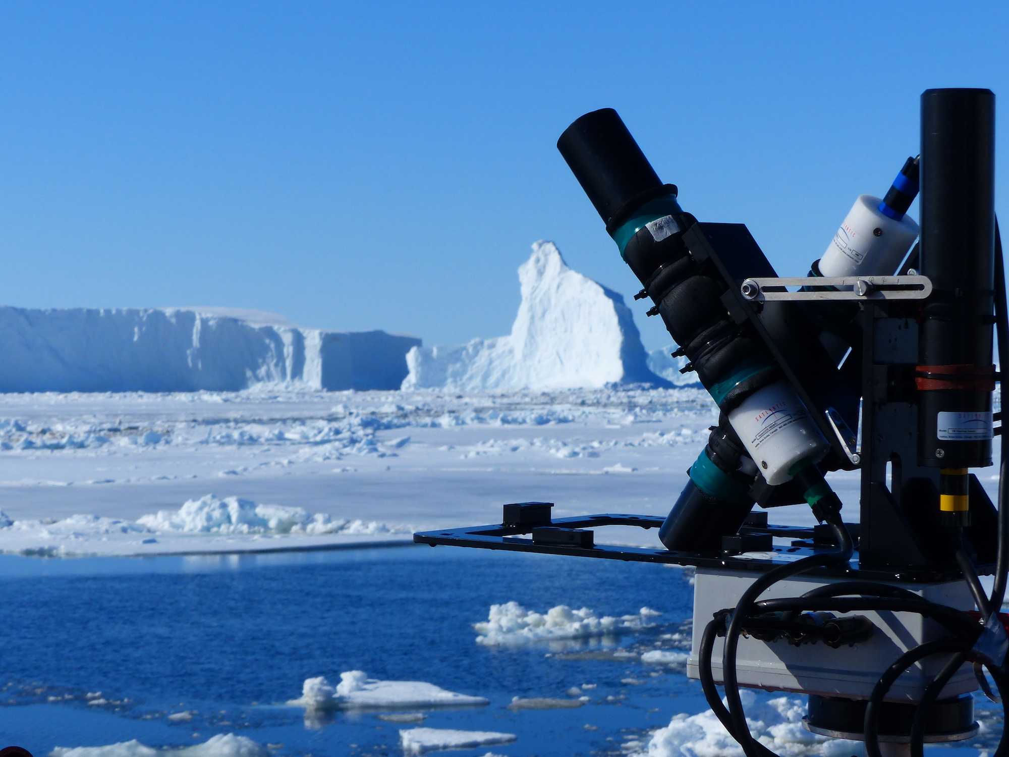
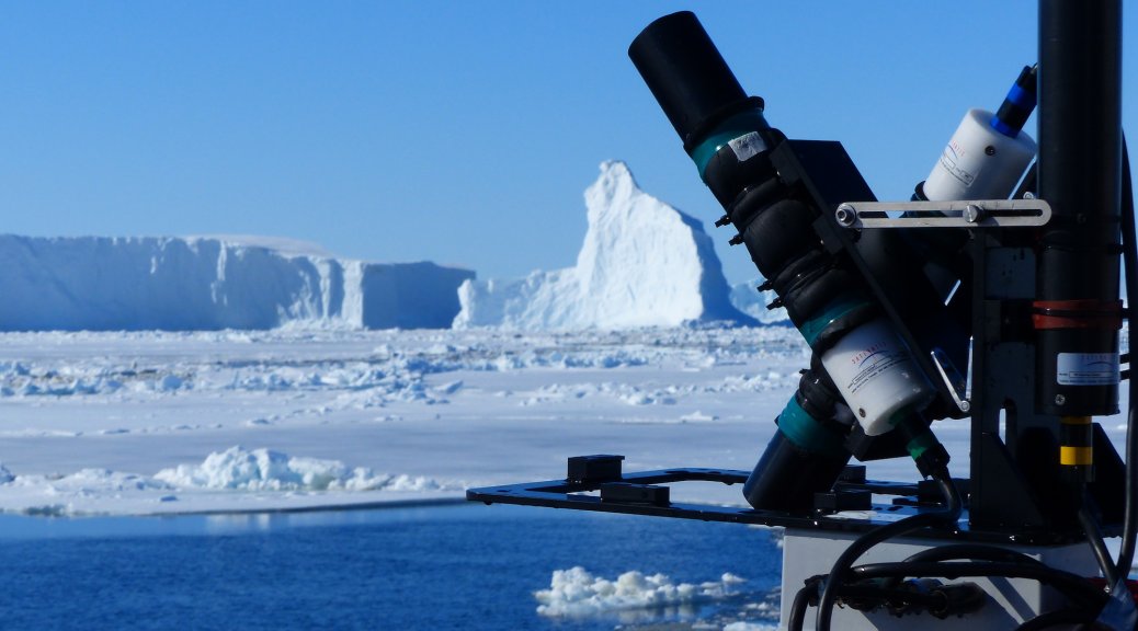
Figure 1: HyperSAS – Credit: Clemence Goyens

On the field, ocean colour can be retrieved in a similar way as the satellite measurements. Aboard the Amundsen, from our departure from Québec till the end of Leg1, the reflectance of the water has been measured with an “Above Water Optical System” with three hyperspectral sensors (referred to as HyperSAS, Fig. 1) mounted on the front deck of the icebreaker. The HyperSAS includes an irradiance and radiance sensor looking up to the sky to measure the downwelling light and a radiance sensor looking down to the sea-surface to measure the light reflected by the water surface in the visible and near-infrared spectral region (400-800nm). By normalizing the light reflected by the water surface by the downwelling light field, we obtain the ‘Remote Sensing Reflectance’ as a function of the wavelength, Rrs(λ).

During Leg1A in the Baffin Bay between 68° and 70° North, Rrs(λ) have been measured along three transects crossing the marginal ice zone (MIZ) allowing to collect data in (1) open waters, (2) along and within the MIZ and (3) within ice cracks in the ice sheets or leads. HyperSAS measurements have been processed and filtered to exclude any Rrs(λ) spectra affected by white caps, large swells and/or rapid changes in shading and illumination conditions as well as ice floes present in the field of view of the sensor. All these artifacts need to be extracted, as these are not directly related to the water column itself and its constituents. Next, each spectrum has been classified according to the optical classification of Melin and Vantrepotte (2015) allowing distinguishing relatively clear waters from turbid waters with higher concentrations of Chla.

Figure 2: Transect and Sentinel2 – Credit: Clemence Goyens

Figure 2 shows the HyperSAS data taken during Leg 1A with a zoom on the three transects crossing the MIZ between June 9th and June 21th (i.e., AB, BC, DC). The figure also includes the ice edge and MIZ as delineated by the U.S. Naval Ice Center (NATICE) and the available Sentinel-2 images for June 16th and 17th.

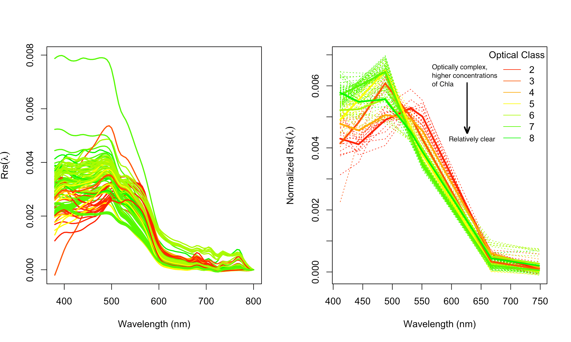
Figure 3: Measured and normalized Rrs(λ) – Credit: Clemence Goyens

Figure 3 shows the measured and the normalized Rrs(λ) (i.e., spectra normalized by the area below its curve). The latter allows highlighting the shape of the spectrum rather than the magnitude. The colors correspond to the optical classes from Melin and Vantrepotte (2015). We found 8 different optical classes in our dataset ranging from optically complex waters with high concentrations of Chla (class 2) to relatively clear waters (class 8). Figure 4 shows how the shape of the water reflectance spectra changes along each transect from sea ice field to open water (transects BA, BC and DC) and for different wavelengths (bleu, green and red). The color of the points in each plot indicates the optical class according to Melin and Vantrepotte (2015). The distance is measured along the transect with 0 corresponding to the ice edge (according to NATICE at the date of measurement). Negative distances correspond to measurements in the ice field left from the MIZ edge while positive distances correspond to the measurements taken in open water. Most spectra show moderately to mesotrophic waters with a peak in the blue spectral region and relatively low concentrations of Chla. However, when crossing the MIZ, Fig. 4 clearly shows the decrease in water reflectance in the blue spectral region and the increase in the green and red spectral region. These results indicate the presence of phytoplankton blooms along the MIZ confirming the existence of “Green Edge”…. and “Green Leads”!

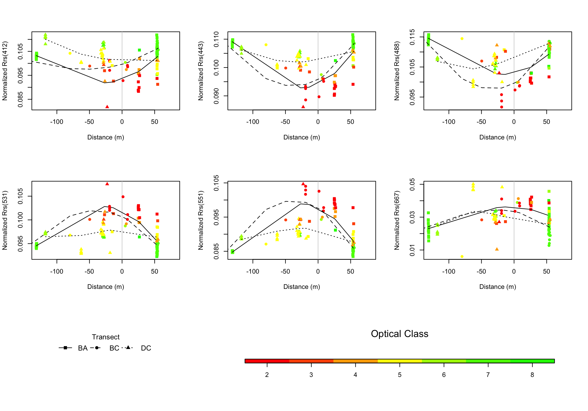
Figure 4: Shape of the water reflectance spectra changes along each transect from sea ice field to open water (transects BA, BC and DC) and for different wavelengths (bleu, green and red) – Credit: Clemence Goyens

However, when crossing the MIZ, Fig. 4 clearly shows the decrease in water reflectance in the blue spectral region and the increase in the green and red spectral region. These results indicate the presence of phytoplankton blooms along the MIZ confirming the existence of “Green Edge”…. and “Green Leads”!